Understanding Dynamic Light Scattering
When in solution, macromolecules are buffeted by the solvent molecules. This leads to a random motion of the molecules called Brownian motion. For example, consider this movie of 2 µm diameter particles in pure water. As can be seen, each particle is constantly moving, and its motion is uncorrelated with the other particles. (Movie courtesy of Dr. Eric R. Weeks, Emory University).
Brownian motion.
As light scatters from the moving macromolecules, this motion imparts a randomness to the phase of the scattered light, such that when the scattered light from two or more particles is added together, there will be a changing constructive or destructive interference. This leads to time-dependent fluctuations in the intensity of the scattered light (Fig. 1).
In dynamic light scattering (DLS), the time-dependent fluctuations in the scattered light are measured by a single photon counting module. The rate of fluctuations is directly related to the rate of diffusion of the molecule through the solvent, which is related in turn to the particles' hydrodynamic radii. Smaller particles diffuse faster, causing more rapid fluctuations in the intensity than larger particles. Therefore, the fluctuation in light intensity contains information about the diffusion of the molecules and can be used to extract a diffusion coefficient and calculate a particle size.
DLS is employed by the DynaPro™ NanoStar™, the DynaPro™ Plate Reader, the ZetaStar™ and the WyattQELS™ module for MALS detectors to determine the effective particle size. The analyte’s translational diffusion coefficient, Dt, is obtained by automated nonlinear least squares fitting of the autocorrelation function that quantitatively describes the measured time-dependent fluctuations in light scattering intensity. The analysis is done directly in the accompanying DYNAMICS™, DYNAMICS Touch™ or ASTRA™ software. A typical autocorrelation function for a monodisperse sample is shown in Fig. 2.
The Stokes-Einstein equation then gives the hydrodynamic radius, Rh, (Fig. 3) corresponding to the measured Dt:
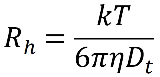
where k is Boltzmann's constant, T is the temperature in K, and h is the solvent viscosity.
Different sizing techniques, e.g., DLS, small angle X-ray scattering, microscopy, and molecular modeling may report different types of radii. It is therefore important to know how a reported “size” was determined and whether it refers to the radius or diameter of the molecule. The Rh measured by DLS is the radius of a hard sphere with the same diffusion coefficient as the sample. Other measures include Rg (the radius of gyration, or root-mean-square radius, obtained by e.g., MALS), Rvol (the radius of a hypothetical sphere that occupies the same volume as the macromolecule), and RRot (the radius subtended by rotating the macromolecule). Fig. 3 illustrates how these different measures compare for the compact, globular protein lysozyme.
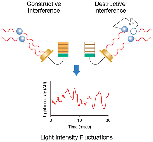
Figure 1. Brownian motion results in measurable fluctuations in the light intensity over time.
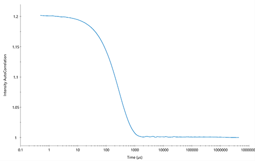
Figure 2. Autocorrelation function for a monodisperse sample with 50 nm Rh particles.
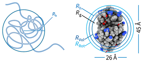
Figure 3. (Left) Rh is the radius of a hard sphere with the same diffusion coefficient as the sample. (Right) Compact molecules, e.g., globular proteins such as lysozyme, generally have Rg < Rh.
Analyzing Particle Size Distributions
Batch DLS can determine size distributions and the presence of multiple populations in a sample without the need for chromatographic separation, making it an excellent tool for rapid quality control and high-throughput screening of large numbers of samples. Such batch measurements of samples with a distribution of Rh and a corresponding distribution of diffusion times will yield autocorrelation functions described by the sum of the autocorrelation functions of all particle species in the sample weighed by their light scattering intensities. Wyatt Technology’s DYNAMICS™, DYNAMICS™ Touch™ and ASTRA™ software programs incorporate two methods for extracting additional information from batch measurements of such complex samples: Cumulants and Regularization (Fig. 4).
The Cumulants method assumes one population of particles with a single average diffusion coefficient and a single standard deviation about that average. The algorithm can fit monomodal samples that are monodisperse or polydisperse (Fig. 4), such as nanoparticles or protein samples with populations of monomers, dimers and small oligomers.
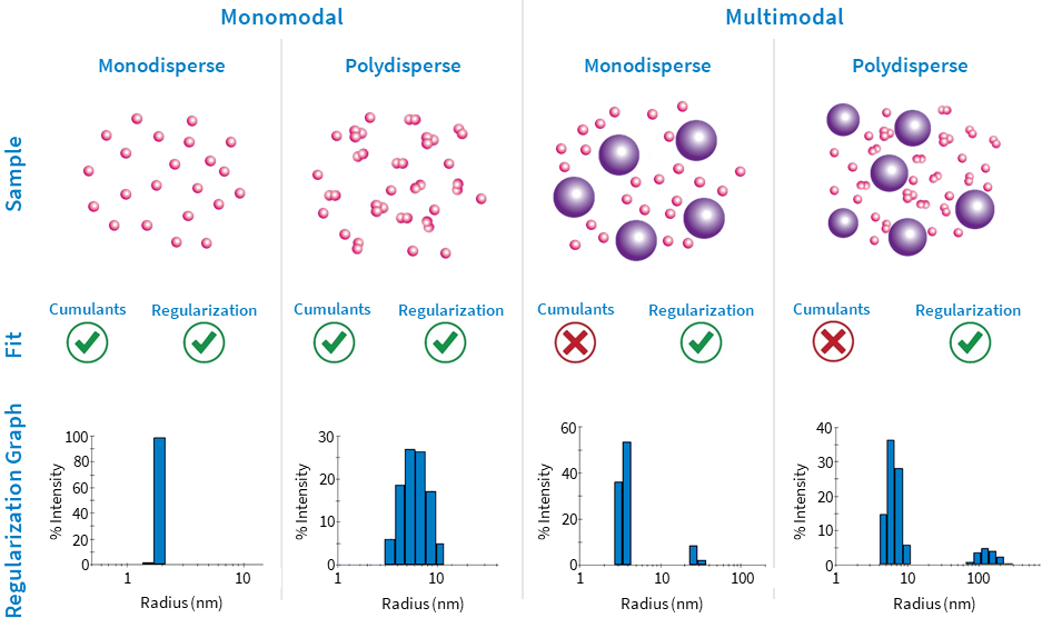
Figure 4. Types of samples, the fits applicable to these samples and a typical Regularization graph are shown.
The Regularization method, in contrast, assumes the presence of any number of populations of particles, each with its own diffusion coefficient, polydispersity, and standard deviation (i.e., the underlying distribution of Rh is smooth). Regularization can resolve species that differ by more than 3-5 times in size. This makes it the method of choice for identifying large aggregates and insoluble species in protein samples.
For each peak or species, Regularization analysis provides a wide range of metrics, including:
- a size distribution histogram (examples shown in the bottom row of Table 1)
- mean radius
- % polydispersity
- molar mass estimated from the measured radius (Mw-R)
- the relative light intensity scattered by each population (%Intensity), estimated relative amount of mass (%Mass) or number of particles (%Number).
Cumulants and Regularization fits and their corresponding residuals are displayed instantly following data acquisition in DYNAMICS and DYNAMICS Touch (Fig. 5), along with an automatic data quality assessment. This allows the user to quickly determine which measurements meet data quality standards, which need to be scrutinized or revisited, and which method provides the best fit.
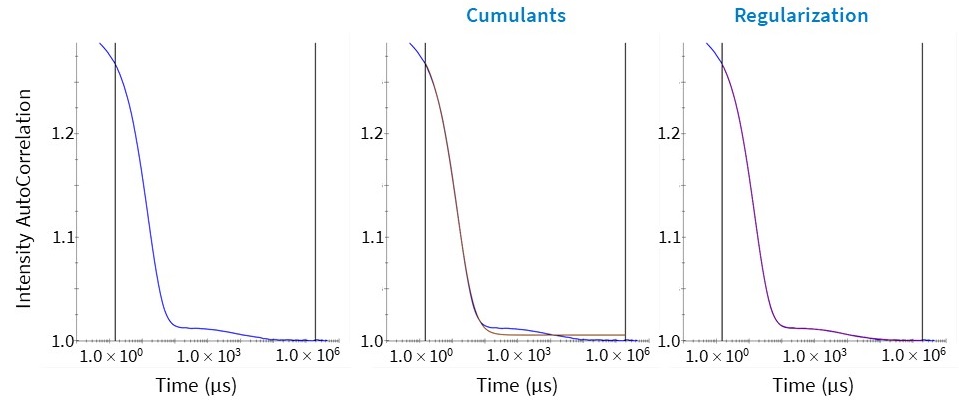
Figure 5. (Left) Autocorrelation function of a multimodal sample (blue). (Middle) The Cumulants fit to the autocorrelation function (brown). (Right) The Regularization fit to the autocorrelation function (purple.) The Cumulants fit does not fit the autocorrelation function well for this multimodal sample.
Measuring Nanoparticle Concentration
Taking advantage of the determination of hydrodynamic size from the diffusion behavior, and the total scattered intensity, another important property can be measured: the concentration of nanoparticles, N.
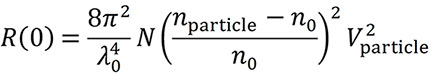
The calculation requires the particle’s volume V and refractive index nparticle, and the refractive index of the solvent n0. The assumption of a user-specified shape model (e.g., uniform sphere or coated sphere) is also required. Then the diffusion coefficient may be interpreted to obtain a dimension such as radius, from which the volume of the particle is calculated (Fig. 6). The refractive index of the particle’s constituent material may be found in the literature. The particle concentration per unit volume, N, can then be determined from the light scattering intensity quantified as the excess Rayleigh ratio at angle zero and the following equation (Van Holde, K. E. Physical biochemistry. Prentice-Hall, 1971):
The maximum Rh for concentration measurements are 160 nm for the DynaPro Plate Reader and 175 nm for the NanoStar. Particles with larger sizes and more complex shapes require multi-angle light scattering (MALS) and can be probed with the Eclipse™ FFF-MALS instrument.
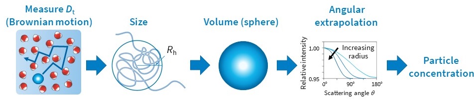
Figure 6. DLS can be used to measure the particle concentration in a sample.
Characterizing Intermolecular Interactions
Nonspecific intermolecular interactions are found throughout nature and have multiple physical origins, including electrostatic attraction and repulsion, hydrophobic and excluded volume effects, and induced dipoles. Interactions can be attractive or repulsive, and are of interest in the formulation of biotherapeutics.
Both the DynaPro NanoStar and DynaPro Plate Reader can quantify macromolecular interactions with DLS and/or SLS. DLS assesses nonspecific interactions and colloidal stability via the diffusion interaction parameter kD. SLS quantifies the second virial coefficient (A2). Both kD and A2 represent complementary metrics of the solute-solute interaction in a specific solvent, and are useful both for understanding interactions and for ranking formulations.
In an ideal dilute solution, the diffusion coefficient (Dt) measured by DLS is not dependent on solute concentration. As concentration increases, the solution becomes less ideal, and a first-order expansion is performed; the diffusion interaction parameter, kD (with units of mL/g), is the first-order correction to the diffusion coefficient as follows:
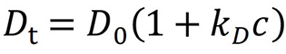
kD is determined by measuring the diffusion coefficient as a function of concentration, in the concentration range where the first-order approximation applies (typically 1 – 10 mg/mL).
Attractive interactions (kD < 0) cause an apparent decrease in Dt and an apparent increase in Rh, while repulsive interactions (kD > 0) cause an apparent increase in Dt and an apparent decrease in Rh (Fig. 7). Molecules behaving as hard spheres for which A2 is close to the excluded volume value typically have kD values between 0 and 5 mL/g.
The diffusion interaction parameter is not a purely thermodynamic quantity – it combines thermodynamic and hydrodynamic contributions. For a purely thermodynamic quantity describing colloidal interactions, the second virial coefficient is commonly explored.
The second virial coefficient, A2, obtained by SLS and MALS via measurements of scattered intensity versus concentration, also reports on solvent-dependent macromolecular self-association and colloidal stability. Specifically, attractive interactions (A2 < 0) cause the scattering intensity to increase faster than linear and yield an apparent increase in molar mass, and repulsive interactions (A2 > 0) cause the scattering intensity to increase slower than linear and yield an apparent decrease in molar mass (Fig. 8). At low concentrations typical of chromatography, the effect of A2 is negligible, and A2 can be set to 0 for data analysis.
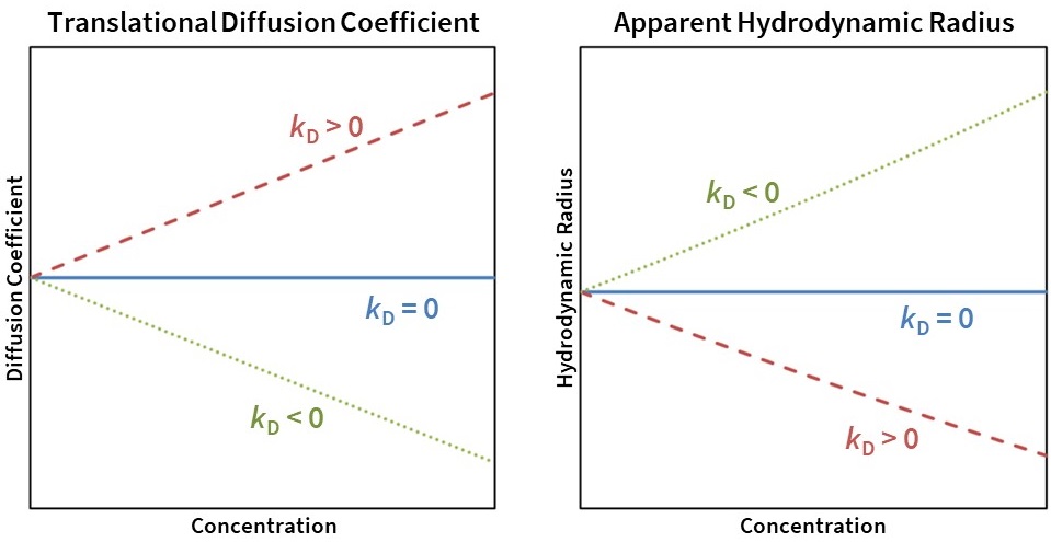
Figure 7. Translational diffusion coefficient (left) and apparent Rh (right) as a function of concentration for kD = 0 (solid blue line), kD> 0 (dashed red line), and kD < 0 (dotted green line).
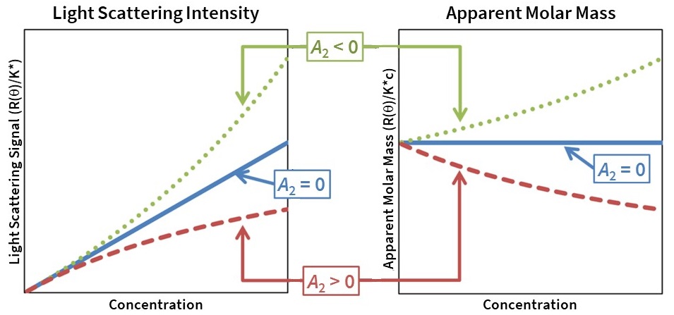
Figure 8. Light scattering intensity (left) and apparent molar mass (right) as a function of concentration for A2 = 0 (solid blue line), A2 > 0 (dashed red line), and A2 < 0 (dotted green line).
Understanding the Autocorrelation Function
In DLS, the fluctuations in light intensity measured over time are quantified via a second order correlation function g(2) (τ). The function of intensity is shifted by a delay time (τ) and the autocorrelation function g(τ) is calculated. Qualitatively, the autocorrelation function is a measure of how similar the intensity function is to itself when shifted by time τ. As the value of τ increases, the function reaches a baseline of 1.
More specifically, and as described in various light scattering texts (cf. Chu, B. Laser Light Scattering: Basic Principles and Practice; Academic Press: Boston, 1991), the correlation function for a monodisperse sample can be analyzed by the equation:
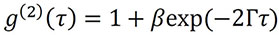
where β is the correlation function amplitude at zero delay, Γ is the decay rate, and the baseline of the correlation function relaxes to a value of 1 at infinite delay.
DYNAMICS and ASTRA use a nonlinear least squares fitting algorithm to fit the measured correlation function to equation 2 to retrieve the correlation function decay rate Γ. From this point, Γ can be converted to the translational diffusion coefficient Dt for the particle via the relation:

Here, q is the magnitude of the scattering vector, and is given by:
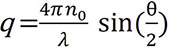
where n0 is the solvent index of refraction, Λ0 is the vacuum wavelength of the incident light, and q is the scattering angle.
Finally, the diffusion coefficient can be interpreted as the hydrodynamic radius Rh of a diffusing sphere via the Stokes-Einstein equation:
where k is Boltzmann's constant, T is the temperature in K, and h is the solvent viscosity (Fig. 3).